- is a specific kind of diagram which is named in honor of Johann Christian Lange’s logic machine ‘Cubus Logicus’ (1714)
- combines features of Euler-type, Venn-type, tree diagrams and esp. square of opposition
- can be applied to ontology engenering and used as an inference engine
- is based on an idea that is as simple and user-friendly as possible
Some information of how to use CL
- Lemanski J. (2018) Calculus CL as Ontology Editor and Inference Engine, in: Chapman P., Stapleton G., Moktefi A., Perez-Kriz S., Bellucci F. (eds) Diagrammatic Representation and Inference. Diagrams 2018. Lecture Notes in Computer Science, vol 10871. Springer, Cham
- Jansen, L. & Lemanski, J. (2020) Calculus CL as Formal System, in: Pietarinen, A.-V., Chapman, P., Bosveld-de Smet, L., Giardino, V., Corter, J., Linker, S. (Eds.): Diagrammatic Representation and Inference11th International Conference, Diagrams 2020, Tallinn, Estonia, August 24–28, 2020, Proceedings. Springer, Cham.
- Lemanski, J. (2020) Calculus CL – From Baroque Logic to Artificial Intelligence, in: Logique & Analyse 249-250.
- Schang, F. & Lemanski, J. (forthc.) A Bitstring Semantics for Calculus CL, in: Vandoulakis, I.: The Esoteric Square of Opposition. Birkhäuser, Basel.
- Lemanski, J. (forthc.) Extended Syllogistics in Calculus CL, in: Journal of Applied Logics.
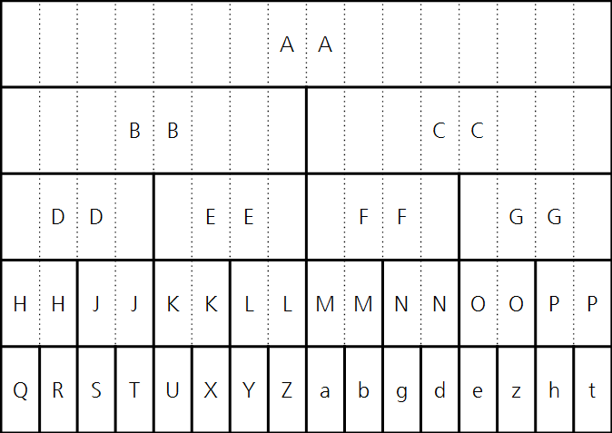
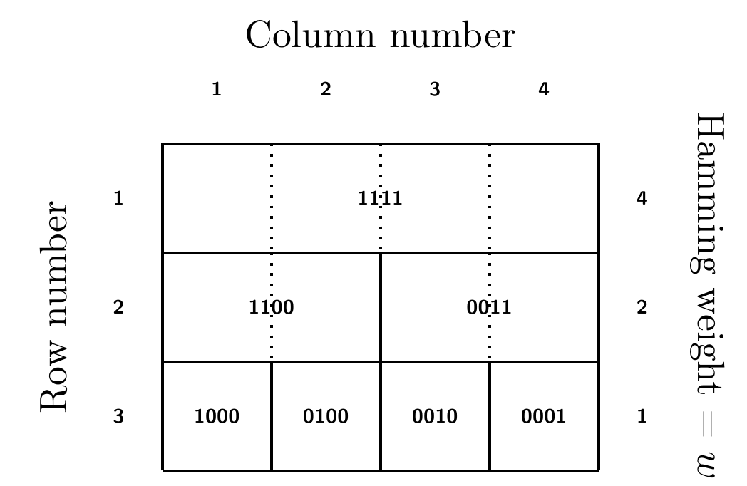
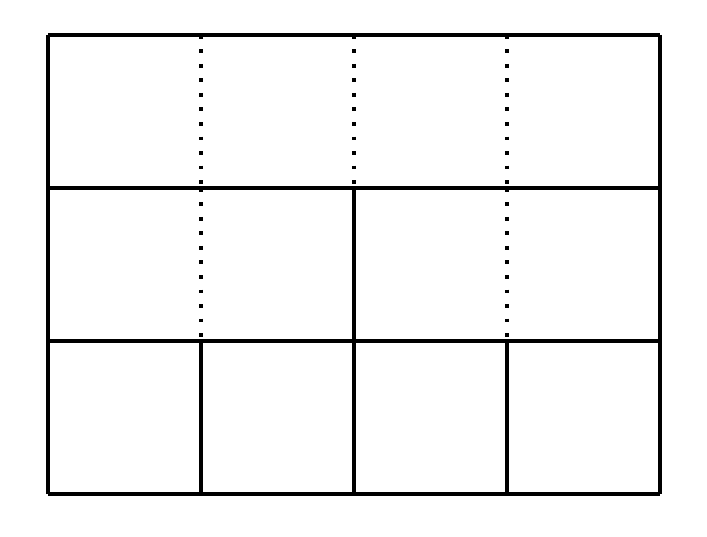
Some printable versions of minimal CL diagrams:
- with 16 Basics (and letters)
2. with 4 Basics (and bitstrings)
3. with 4 Basics (without bitstrings)
An example for Tikz users
\documentclass[10pt,a4paper,draft]{article}
\usepackage[utf8]{inputenc}
\usepackage[T1]{fontenc}
\usepackage{tikz}
\begin{document}
\begin{tikzpicture}
%example content elements
%an arrow
%\draw [->] (2.5,0) -- (2.5,2);
%shading
%\filldraw[fill=gray, draw=gray] (0,1) rectangle (2,2);
%tensors
%\draw[solid]
%(0.5,0.5) node {$\bigotimes$}
%-- (1.5,1.3) node {$\bigotimes$};
%The basics (+0.05 on x per column)
%horizontal lines bottom and top
\draw [line width=0.7pt](0,0) -- (4,0) (0,1) -- (4,1) ;
%vertical solid lines (+1 on x)
\draw [line width=0.7pt](0,0) -- (0,1) (1,0) -- (1,1) (2,0) -- (2,1) (3,0) -- (3,1) (4,0) -- (4,1);
%
%Level 1
%horizontal line top
\draw [line width=0.7pt] (0,2) -- (4,2);
%dotted vertical lines (+1.0 on x)
\draw [dotted,line width=0.7pt] (1,2) -- (1,1) (3,2) -- (3,1);
%solid vertical lines (+1.0 on x)
\draw [line width=0.7pt] (0,1) -- (0,2) (2,2) -- (2,1) (4,2) -- (4,1);
%
%Level 2
%horizontal line top
\draw [line width=0.7pt](0,3) -- (4,3);
%dotted vertical lines (+1 on y)
\draw [dotted,line width=0.7pt] (1,3) -- (1,2) (2,3) -- (2,2)(3,3) -- (3,2);
%solid vertical lines (put every 2nd svl of level 1 in dvl of level 2 & +0.5 on y)
\draw [line width=0.7pt] (0,2) -- (0,3) (4,3) -- (4,2);
%
%Level 3
%horizontal line top
%
%the enviroment
\node at (2.0,4.0) {Column number};
\node at (-1.0,1.5) [rotate=90]{Row number};
\node at (5,1.6) [rotate=270]{Hamming weight = $w$};
%left to right, the columns
\node [font = \sffamily\bfseries \tiny] at (0.5,3.5) {1};
\node [font = \sffamily\bfseries \tiny] at (1.5,3.5) {2};
\node [font = \sffamily\bfseries \tiny] at (2.5,3.5) {3};
\node [font = \sffamily\bfseries \tiny] at (3.5,3.5) {4};
%
%the rows
\node [font = \sffamily\bfseries \tiny] at (-0.4,0.5) {3};
\node [font = \sffamily\bfseries \tiny] at (-0.4,1.5) {2};
\node [font = \sffamily\bfseries \tiny] at (-0.4,2.5) {1};
%
%the levels
\node [font = \sffamily\bfseries \tiny] at (4.4,0.5) {1};
\node [font = \sffamily\bfseries \tiny] at (4.4,1.5) {2};
\node [font = \sffamily\bfseries \tiny] at (4.4,2.5) {4};
%the bitstrings
%Basics
\node [font = \sffamily\bfseries \tiny] at (0.5,0.5) {1000};
\node [font = \sffamily\bfseries \tiny] at (1.5,0.5) {0100};
\node [font = \sffamily\bfseries \tiny] at (2.5,0.5) {0010};
\node [font = \sffamily\bfseries \tiny] at (3.5,0.5) {0001};
%
%Level 1
\node [font = \sffamily\bfseries \tiny] at (1,1.5) {1100};
\node [font = \sffamily\bfseries \tiny] at (3,1.5) {0011};
%
%Top-Level
\node [font = \sffamily\bfseries \tiny] at (2,2.5) {1111};
\end{tikzpicture}
\end{document}